CCI – Centre for Cell Imaging

Leica Stellaris Falcon

Microscope BrandBuildingRoom
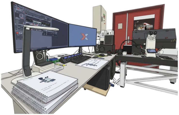
Leica Confocal Androclus CCI O.124A
Reservation Link Specs Download Quickstart ManualLabJounal Recording sheet (setting-file – rank)
Objective List
Position Magnification NAImmersion mediumWD (mm)FOV (um)BrightnessCorr CollarRemark
150.15 air13
2100.4air2.56
3200.7air0.62
4401.3oil0.24
5631.4oil0.14
6
Light Sources
EL6000
White Light Laser (440-790 nm)
Diode Laser (405 nm)
Diode Laser (448 nm)
Diode Laser (488 nm)
Fluorescence Filters
FilterDye
1DAPI
2FITC
Prism / AOBSfree range 450 – 850 nm
Detectors
DetectorsPosition
HyD-S1
HyD-X2
HyD-S3
HyD-X4
HyD-R5

Functional Modalities
Brightfieldx
DICx
Phase Contrast
Wide Field Fluorescencex
TIRF
Confocalx
Multiphoton
Photomanipulationx
Live Cell Imagingx
LifeTime Measurementx
SMLM (PALM/STORM)

Quickstart Manual

Prepare

  • Make notes of settings, rank your nicest images (link for a CCI-prepared template)
  • Configuration tab: Bit depth 8<>16 bit, Glow Over, HyD’s in Count mode recommended
  • Is optimal pixel size required for the experiment? Choose suited Objective and adjust pixel size to meet Nyquist criteria only when you need it
  • Decide if, and which detector setting uses the transmitted light detection
  • Know the dyes in your samples (spectral, lifetimes if available, stability)
    • Excitation/Emission spectra can be shown/uploaded in LAS-X dye database (Configuration tab)

File Save Preparation and Focus on cells

  • Save Preparation: presets File Naming and file location
    • <.xlef> = lif+ extended metadata
    • In <New Project Defaults> set Project name: <YYYYMMDD_#UID-RefID (link to LabJournal)>
    • set <User defined name> #UID-RefID_TXT-describes-experiment_Channel-desciption
    • NO special characters (!@#$%^&*(){}?|\/=][><~`”;:) or SPACES, < 256 characters (with folder names)    
    • <Autosave> to save multidimension data during acquisition (tick <OFF> while tweaking)
    • File Location: subfolders on E:\ImageDATA\<USER>\<DATE: YYYMMDD>
    • Make a <New Project> when switching samples (LAS-X add counters, Well-/ROI-name), re-save list frequently.
  • Focus on cells
    • Transmission images usually work fine, low Mag 5x/10x, find a cs/well edge and move to cells, use a simple method or view by eye

Setting the detection filters (Image Compass)

  • Start in Acquisition Mode (in Viewer: Split Channel / Activate Intensity Histogram)
  • Optimize detector settings: Reuse/Create a detection sequence from file metadata or saved setting file => CHECK before use (LabJournal notes – link)
    • Hardware: Objective, filter ranges, laser (l, power), HyD (type, mode, Gain, AI denoise),
    • Acq Settings: Pixel Size (Format & Zoom), Pix Dwell time (Speed-Galvo/Res, Bi-Dir), Pinhole, Acc/Avg, Z step, Z  range, t interval-duration
  • Search Dye, select and drag it onto the preferred HyD Detector (or drag onto empty space for automated setting), repeat for every dye
    • Figure1: HyD propertiesChoose optimal HyD Type for Dye (order S1>X2>S3>X4>R5, start at shortest wavelength)
  • Choose sequential mode to record dye (sets)
    • <+> Add a detector group, Ms(R) to reset a group
    • Line recommended, Frame allows different Acc or Avg per group  
    • <Uncheck> to temporarily skip its acquisition
    • Avoid Dye Assistant, it resets filter ranges and does not include the HyD-R detector of the system (use it to get dye combination hints, do not <Apply>)
  • Choose mode of the HyDs (analog/digital/photon count (FLIM)/reflection)
  • Set Emission Filter Slider range
    • Fit emission spectra (shallow => ¯ Crosstalk & ¯ Signal), tweak Yield/Crosstalk by shifting the range
    • Ms(Clk)2 on slider to type l-limits or Clk-n-Drag ends
    • No overlap with laser line (>8nm away) & AFC aborts when a filter ³750 nm
  • Set Excitation Laser l
    • Fit excitation spectra – reduce Crosstalk by shifting from optimal, use PanelBox or Ms(Clk)2 the line to type
    • Inspect bleed/Crosstalk by varying Laser Intensity for the ‘donor’ channel, Intensity of the ‘acceptor’ Channel should not change, best evaluated in Viewer with Split channel & Histogram activated
    • Interactive elements open different setting GUIs (see numbered items in figure 2)
  • Choose group that generates the Transmission channel (TransPMT >> <ON>, set its Gain/Offset)
  • Set LUTs or channel coloring and save the setting in your data folder
    • Recommend to choose color blind-friendly sets that work well for presentation via beamers etc.)
    • Blue> Cyan, Red> Orange/Yellow, NIR> Magenta, TM > Grey; Explore Inverted for weak/sparse labels
  • Figure 2: Interactive GUI elements in the Image Compass

Use CCI form (on desktop or CCI website) dedicated to structure documentation of settings, save as: Setting-UID in your data folder before filling the form. Setting comments, for example Z range, Z step, T Interval

Tweak Acquisition Scanning parameters:

Start/Stop scanning

  • <FAST Live> to scan quickly (fast setting tweakable, it scans only the activate -white marked- Detector Group)
  • <Live> scans all channels as set (starts by Panelbox <Right Button>)
  • <Capture> takes image channels and omits other dimensions<START> records all set dimensions
  • Compare images in <Viewer> by <+> to add another Project Image, linking synchs Zoom/Intensity changes, <X> to remove a parallel view

Acquisition Parameter setting

  • Laser Intensity (use the Panel Box <Smart Intensity> or Ms(Clk)2 line to type)
  • Scan Acquisition mode XY
    • Do not oversaturate: Bit type intensity maxima (8b>256, 16b> 65536), use Glow-Over LUT in viewer to evaluate
    • <Zoom in> prompts to make a ROI and Zoom into it
    • <Bidirectional X> scan @ double speed but striping/doubling artefacts can occur (changing with zoom, speed>700, format change etc.), it needs manual Phase-X correction
    • <Format> & <Zoom Factor>  define XY Pixel Size (diffraction limit or not)<Speed> defines Pixel Dwell Time: slower => signal­ , the <Resonance Mode> locked high speed: needs higher laser powers, and avg/acc to improve S/N
    • <Pinhole> defines along with l Optical section & Z step size (choose Airy 1 for the most important channel wlem)
    • <Rotation> orientate sample to optimally fit field
  • Figure 3: Acquisition Scanner Settings
  • Detector setting – signal pooling
  • Define Multidimensional imaging (Z, t, position, etc.=> Select Detection mode)
  • Use <Navigator> to <Align> and use preset Carriers or define ROIs/positions.
  • Check focus control (AFC, Autofocus in noise, make Focus Map in Navigator)
  • Check timing

Using Navigator: Positions – Carrier – ROI Sections

Many of the acquisition GUI is available in the <Navigator> as well in grouped GUIs. Beam Path= image Compass, Scan Mode = XY scan parameters, Z stack, Time, positions GUIs are activated in the <Toolbar>. Generally, preparing imaging is easiest done in the acquisition tab while overview/position/tile/ROI functions are done in the navigator.

  • Ms(Clk)2 move to position and makes <Preview> image, Ms(Wheel) to Zoom.
    • <AFC> performs quite well in <Spiral Scan>, Ms(R) to select variants of the spiral scan
    • Avoid LUT pileup of all (tiles and) previews in the images listing by unchecking or deleting unnecessary previews/Tiles. Setting LUT for the active FOV is quite difficult otherwise.
    • <Split Channel View>  for active position FOV, a GUI offers options to overlay. Switch back to <Stage Overview> to resume tile actions
    • <Task List> Check/Unchecking ROIs/wells can be per group as well. <START> will only record checked <Tasks>
    • <Save Overview…> saves the checked pre/over-views in <Projects>
    • <Mosaic Merge> generates a single large file in <Projects>

Figure 4: Navigator

Focus MAP

  1. Make Spiral overview (low mag)
  2. Select ROI with drawing tools
  3. < Check > keep Drawing Tool active
  4. <+F> to set focus XY position (remove by Select> Delete)
  5. <+AF> to use in Timelapse / Stage (set <..on Demand> – everty xth in time / position)
  6. <Focus Map…> to activate dialog and list XY
  7. <Set Z> Manual /  Autofocus for active or all point(s) => Values Z/AFC are shown
    • OPTION: Shift Entire MAP in Z by defined offset (workaround to do asymmetric stacking)
    • CONTEXT Menu: Subtract Tool / Group Scan Regions / Paste Regions in Chambers etc.

Lightning Mode: Automate parameter setting to perform live deconvolution

  • Autoparameter setting (unchain to adjust setting)
  • LAS-X gets immersion media refractive index, estimates of imaging depth aberrations and psf’s for the channels from metadata
  • Adaptive  = generally better than Global
  • Set the mounting media correctly (see table below)
    • Deconvolution is also available in the Process tab

Figure 5: Lightning mode GUI -refractive index list

Auto ParameterSpeed<>Resolution
Pinhole(AU)~1<>up to 0.3
Pixel/Z-step..<>Nyquist for given Pinhole
Speed ..<>Decreases to improve light collection
Line Avg ~1<>Increases for better S/N
HyD gain Up to You <>Up to You
Laser % Up to You>>Up to You
NameRefractive index
VectaShield Vibrance 1.47 (cured)
VectaShield Plus 1.45
VectaShield Hardset1.46 (cured)
VectaShield1.45
SlowFade Gold1.42
SlowFade Glass1.52
SlowFade Diamond1.42
ProLong Gold1.46
ProLong Glass1.51
Prolong Diamond1.46
Mowiol1.42
Fluoromount G1.42
Entellan1.49
DPX1.52
Canada Balsam1.52

Tau Separation: lifetime (t) isolation or gating (Dt >1 ns)

Average Photon arrival time per pixel => assign Pix to an avg t class

Different options to extract / highlight Tau from images

  • Prerequisites:
    • WLL (OPTION: notch filtered reference lines) / TauContrast <ON> / HyD in count mode
    • WLL pulse frequency should accommodate 3-4x the expected longest lifetime
    • Maximal Photon count rate should be Pulse rate @ 0.1 / laser pulse (Pixel Int Histo)/ 0.37 with Photon count filter
    • Tau output images are kept as separate channels in <Projects>
  • TauContrast (analyse lifetime components in an emission block) > Intensity
  • TauScan (set nr of images to extract t -spieces)
    • OUTPUT: nr series with t-range/nr, => spot the peak intensities in the image range
  • GateScan (nr of preset Gates to estimate t-species): <+> to add onther channel and slider set to define bounds
    • OUTPUT: series of defined t-”bins” => spot differences in the extracted images
  • TauGating:  Set t range based on Tau/Gate-Scan to put in a channel (unchecked range(s) will not be recorded => omit reflections, autofluorescence)
    • OUTPUT: Tau Images with selected t characteristics (and omitted t species from the recorded images)
  • TauSeparation (use t estimates from Tau/Gate-Scan, <+> and define in slider, or allow algorithm to extract them, )
    • OUTPUT: Tau Images with defined t characteristics